An Information-Hydrodynamical View of Quantum Mechanics
An intuitive view of the Madelung equations through Information-Hydrodynamics
Background
Every now and then, I read about something so neat I feel compelled to write about it. Occasionally, I stumble on something myself which I feel the need to share. (Un?)luckily for the readers, today is such a day!
This post concerns an optimal-transport and information-geometric view of the hydrodynamical formulation of the Schrödinger equation, known as the Madelung equations.
A particularly clean connection between optimal transport and the Madelung equations was described by von Renesse in An Optimal Transport View of Schrödinger’s Equation.
In Appendix C of a recent preprint with Boris Hanin, The Score Hamiltonian: Mapping Diffusion Models to Adiabatic Transport, we observed that the ground-state factorization underlying the Score Hamiltonian also yields an exact real-time decomposition of the Madelung energy into a relative Fisher information and a phase kinetic energy (Proposition C.2). The paper’s main focus is the correspondence between score-based diffusion or time-inhomogeneous Langevin sampling and imaginary-time adiabatic transport of instantaneous ground-states (which I might post about in the future). This blog post instead surfaces the complementary real-time, information-hydrodynamical interpretation.
For two absolutely continuous probability densities
\[\mu,\nu\in\mathcal P_{2,\mathrm{ac}}(\mathbb R^d),\]denote their relative Fisher information by
\[I_{\textrm{Rel}}(\mu\|\nu) = \int_{\mathbb R^d} \mu(x) \left\| \nabla\log\mu(x)-\nabla\log\nu(x) \right\|^2\,dx.\]Let
\[\hat{H} = - \frac{\hbar^2}{2m} \nabla^2 + V\]be a time-independent Hamiltonian on $L^2(\mathbb R^d)$ with a strictly positive ground-state
\[\psi_{0}=\sqrt{\rho_{0}}, \qquad \hat{H}\psi_0 = E_0 \psi_0 .\]From this point onward, we absorb the physical prefactor into the notation and write
\[I(\mu\|\rho_{0}) := \frac{\hbar^2}{8m} I_{\textrm{Rel}}(\mu\|\rho_{0})\]Thus, $I(\mu|\rho_{0})$ denotes the relative-Fisher deformation energy, rather than the unscaled relative Fisher information.
Write a quantum state in density and phase variables as
\[\psi_t=\sqrt{\mu_t}\,e^{i\phi_t/\hbar},\]with hydrodynamical velocity $u_t = \frac{\nabla \phi_t}{m}$.
Then, wherever the Madelung representation is well-defined, quantum mechanics may be written as the pair
\[\partial_t\mu_t = -\nabla\cdot(\mu_t u_t),\]and
\[\frac{D u_t}{Dt} = -\frac1m \nabla \frac{\delta I(\mu\|\rho_{0})}{\delta\mu}(\mu_t), \qquad \frac{D}{Dt} := \partial_t+u_t\cdot\nabla.\]for $\frac{D}{Dt}$ the material derivative (the classical convective acceleration in fluid mechanics).
The first equation is the classical continuity equation, which transports probability mass with velocity given by the gradient of phase $u_t = \frac{1}{m} \nabla \phi_t $. The second statement is that convective acceleration is generated by the variational gradient of the relative Fisher information between the active Born density $ \mu_t $ and the ground-state density $ \rho_0 $.
This is the fundamental information-hydrodynamical picture.
To see where this comes from, observe that the Hamiltonian conserved by real-time quantum evolution can be written in terms of the relative Fisher information. For
\[\psi_{t} = \sqrt{\mu_{t}}e^{i\phi_{t}/\hbar},\]one has
\[\langle \psi_{t}|\hat{H}|\psi_{t}\rangle-E_{0}=\frac{\hbar^{2}}{8m}\int \left\lVert \nabla \log \mu_t - \nabla \log \rho_{0} \, \right\rVert^{2}\mu_t\,dx + \frac{1}{2m}\int \left\lVert \nabla \phi_t \right\rVert^{2}\,\mu_{t}\,dx.\]In other words,
\[E - E_{0} = \tilde{T}+\tilde{V},\]where
\[\tilde{V} =I(\mu_t \|\rho_{0}) =\frac{\hbar^{2}}{8m}\int \left\lVert \nabla \log \mu_t - \nabla \log \rho_{0} \, \right\rVert^{2}\mu_t\,dx\]is an energy quantifying the deformation of the density $\mu_t$ relative to the ground-state $\rho_0$, while
\[\tilde{T}=\frac{1}{2m}\int \left\lVert \nabla \phi_t \right\rVert^{2}\,\mu_{t}\,dx\]is the kinetic energy carried by the phase $\phi_t$.
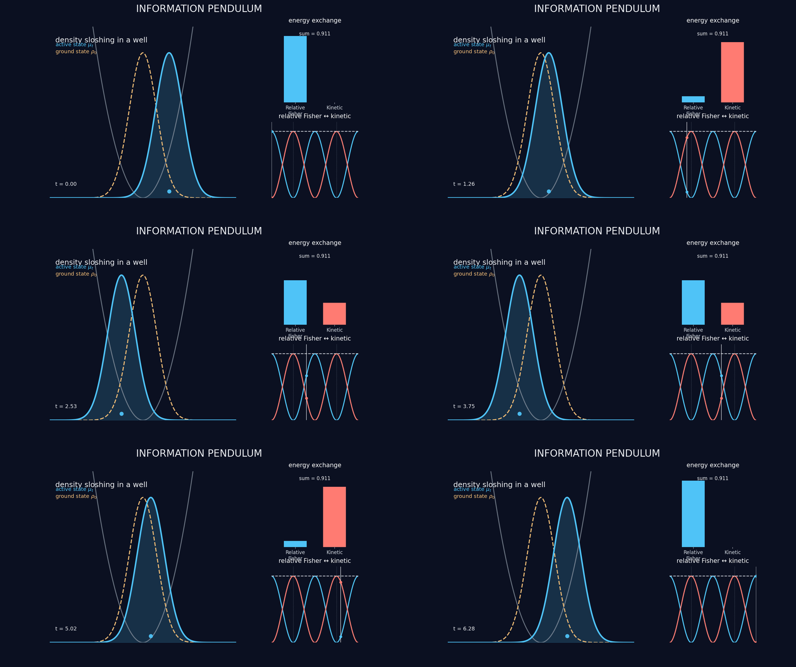
Quantum evolution can therefore be viewed as an information pendulum: energy swings between phase kinetic energy and relative Fisher information deformation energy with respect to the ground-state.
For example, a coherent state of the Harmonic Oscillator has a Gaussian density $\mu_t$ that moves rigidly through the Gaussian ground-state $\rho_0$ (see, e.g.: Video of Quantum HO). When $\mu_t$ swings through the Gaussian ground-state $\rho_0$ its kinetic energy is maximal while:
\[I(\mu_t \|\rho_{0})=0.\]Meanwhile, as the density approaches the edge of the harmonic potential well, its motion slows and the kinetic energy is converted into relative-Fisher deformation energy.
Up to the temporal $\tilde{\phi}_t = \phi_t + E_0 t$ gauge on the phase (and harmlessly suppressing the tilde), taking Euler-Lagrange variations in $ \phi_t $ and $ \mu_t $, as in von Renesse’s formulation, give
\[\partial_t\mu_t = -\nabla\cdot \left( \mu_t\frac{\nabla\phi_t}{m} \right),\]and
\[\partial_t\phi_t+\frac{\|\nabla\phi_t\|^2}{2m} +\frac{\hbar^2}{2m} \left( \frac{\nabla^2\sqrt{\rho_0}}{\sqrt{\rho_0}}- \frac{\nabla^2\sqrt{\mu_t}}{\sqrt{\mu_t}} \right)= 0.\]These are equivalent to the hydrodynamical equations after setting
\[u_t = \frac{\nabla \phi_t}{m}.\]Unlike conventional presentations of Madelung hydrodynamics which invoke both an external potential $ V $ and a quantum potential $Q$ associated with $\mu_t$, this formulation exposes that $ V $ itself can be written in terms of the quantum pressure associated with the ground-state density:
\[V=E_0+ \frac{\hbar^2}{2m} \frac{\nabla^2\sqrt{\rho_0}}{\sqrt{\rho_0}}.\]The effective potential governing the dynamics is thus the difference in quantum pressures
\[\delta P_{Q} := Q_{\rho_0}-Q_{\mu_t}, \qquad Q_\rho := \frac{\nabla^2\sqrt{\rho}}{\sqrt{\rho}}.\]We refer to this, informally, as a quantum pressure gap. Mathematically, it is the effective information potential whose gradient generates the hydrodynamical force of Madelung’s equations.
The Madelung equations
To begin more carefully, let us recall the Madelung equations – introduced by Erwin Madelung in 1926.
Roughly speaking, Erwin Madelung wanted to express the Schrödinger equation in a more intuitive form in which one evolves the Born density itself – something naturally associated with Wasserstein space – rather than only working with an underlying complex amplitude or wave-function in Hilbert space.
The Schrödinger equation evolves a wave-function $\psi_t \in L^2(\mathbb{R}^d)$ according to
\[i\hbar\,\partial_t\psi_t = \left(-\frac{\hbar^2}{2m}\nabla^2 + V\right)\psi_t,\]Born’s rule gives the probability density via the modulus of $\psi_t$
\[|\psi_t |^2 = \mu_t.\]A wave amplitude (*away from nodes!) can be written in polar form as
\[\psi_t = \sqrt{\mu_t} \, e^{i \phi_t / \hbar}\]Substituting this expression into the left-hand side of the Schrödinger equation gives
\[i\hbar\,\partial_t\psi_t=e^{i\phi_t/\hbar}\left( \frac{i\hbar}{2\sqrt{\mu_t}}\partial_t\mu_t-\sqrt{\mu_t}\,\partial_t\phi_t \right).\]For the right-hand side, applying $ -(\hbar^2/2m)\nabla^2 + V $ to $\psi_t = \sqrt{\mu_t}\,e^{i \phi_t/\hbar}$ and collecting terms gives
\[\begin{aligned} \left( -\frac{\hbar^2}{2m}\nabla^2+V \right)\psi_t = e^{i\phi_t/\hbar} \Bigg( & -\frac{\hbar^2}{2m}\nabla^2\sqrt{\mu_t} + \frac{\|\nabla\phi_t\|^2}{2m}\sqrt{\mu_t} + V\sqrt{\mu_t} \\ & -\frac{i\hbar}{m} \nabla\sqrt{\mu_t}\cdot\nabla\phi_t - \frac{i\hbar}{2m} \sqrt{\mu_t}\,\nabla^2\phi_t \Bigg). \end{aligned}\]Setting $ i\hbar\,\partial_t\psi = (-\hbar^2/2m)\nabla^2\psi + V\psi $ and canceling the common factor $ e^{i\phi_t /\hbar} $, the Schrödinger equation is equivalent to
\[\begin{aligned} \Phi = & -\frac{\hbar^2}{2m}\nabla^2\sqrt{\mu_t} + \frac{\|\nabla\phi_t\|^2}{2m}\sqrt{\mu_t} + V\sqrt{\mu_t} + \sqrt{\mu_t}\,\partial_t\phi_t \\ & -\frac{i\hbar}{m} \nabla\sqrt{\mu_t}\cdot\nabla\phi_t - \frac{i\hbar}{2m} \sqrt{\mu_t}\,\nabla^2\phi_t - \frac{i\hbar}{2\sqrt{\mu_t}} \partial_t\mu_t = 0. \end{aligned}\]Separating the real and imaginary parts gives
\[\mathrm{Re}\,\Phi = -\frac{\hbar^2}{2m}\nabla^2\sqrt{\mu_t} + \frac{\|\nabla\phi_t\|^2}{2m}\sqrt{\mu_t} + V\sqrt{\mu_t} + \sqrt{\mu_t}\,\partial_t\phi_t = 0,\]and
\[\mathrm{Im}\,\Phi = -\frac{\hbar}{m} \nabla\sqrt{\mu_t}\cdot\nabla\phi_t - \frac{\hbar}{2m} \sqrt{\mu_t}\,\nabla^2\phi_t - \frac{\hbar}{2\sqrt{\mu_t}} \partial_t\mu_t = 0.\]Multiplying the imaginary part by $-2\sqrt{\mu_t}/\hbar$ and recognizing the resulting expression as a divergence gives
\[\begin{aligned} \partial_t\mu_t &= -\frac1m \left( 2\sqrt{\mu_t}\, \nabla\sqrt{\mu_t}\cdot\nabla\phi_t + \mu_t\nabla^2\phi_t \right) \\ &= -\nabla\cdot \left( \mu_t\frac{\nabla\phi_t}{m} \right). \end{aligned}\]which is the continuity equation.
Dividing the real part by $\sqrt{\mu_t}$ and rearranging gives the quantum Hamilton–Jacobi equation
\[\partial_t\phi_t+\frac{\|\nabla\phi_t\|^2}{2m} +V-\frac{\hbar^2}{2m} \frac{\nabla^2\sqrt{\mu_t}}{\sqrt{\mu_t}}=0.\]Thus, the “ordinary” Madelung equations are:
\[\partial_t\mu_t + \nabla\cdot \left( \mu_t\frac{\nabla\phi_t}{m} \right) = 0,\]and
\[\partial_t\phi_t + \frac{\|\nabla\phi_t\|^2}{2m} + V - \frac{\hbar^2}{2m} \frac{\nabla^2\sqrt{\mu_t}}{\sqrt{\mu_t}} = 0.\]The last term $ - \frac{\hbar^2}{2m} \frac{\nabla^2\sqrt{\mu_t}}{\sqrt{\mu_t}} $ is usually described as the quantum potential (or Bohm potential, following David Bohm’s use of it in his 1952 pilot-wave theory). Informally, it is referred to as a quantum pressure and plays a very special role. In fact, its presence is the sole dividing line between the quantum Hamilton-Jacobi equation (quantum mechanics) and the classical HJ equation (Newtonian mechanics).
Information-Hydrodynamical form of the Madelung equations
Now, suppose our Hamiltonian $ \hat{H} $ has a positive ground-state
\[\psi_0=\sqrt{\rho_0}\]with energy $ E_{0} $. The stationary solution is
\[\psi(x,t) = \sqrt{\rho_{0}}\,e^{-iE_0t/\hbar}.\]Its phase is purely temporal $ \phi_{0}(x,t) = -E_0 t $. Thus,
\[\nabla\phi_{0} = 0, \qquad \partial_t\phi_0 = -E_0 .\]Substituting this stationary solution into the Hamilton-Jacobi equation gives
\[-E_0 + V - \frac{\hbar^2}{2m}\frac{\nabla^2\sqrt{\rho_{0}}}{\sqrt{\rho_{0}}} = 0.\]Thus,
\[V(x) = E_{0} + \frac{\hbar^2}{2m}\frac{\nabla^2\sqrt{\rho_{0}}}{\sqrt{\rho_{0}}} .\]The external potential can thus be reconstructed exactly from the ground-state density up to an additive constant. This direct (one-particle) inversion echoes the Hohenberg-Kohn principle that a ground-state density determines its external potential, although the setting discussed here is considerably simpler.
Substituting this identity back into the Madelung equation, one finds
\[\partial_t\phi_t + \frac{\|\nabla\phi_t\|^2}{2m} + E_0 + \frac{\hbar^2}{2m} \left( \frac{\nabla^2\sqrt{\rho_0}}{\sqrt{\rho_0}} - \frac{\nabla^2\sqrt{\mu_t}}{\sqrt{\mu_t}} \right) = 0.\]Up to the gauge $\tilde{\phi}_t = \phi_t + E_0t,$ (and suppressing tilde from this point onward) this becomes
\[\partial_t\phi_t + \frac{\|\nabla\phi_t\|^2}{2m} + \frac{\hbar^2}{2m} \left( Q_{\rho_0}-Q_{\mu_t} \right) = 0.\]Thus, the usual external potential and active-state quantum potential have collapsed into one relative quantity: the quantum-pressure gap between $\mu_t $ and $ \rho_0 $.
This same structure appears at the level of the (“Information”) Hamiltonian
\[\hat{H}=-\frac{\hbar^{2}}{2m}\nabla^{2}+\frac{\hbar^{2}}{2m}\frac{\nabla^{2}\psi_{0}}{\psi_{0}}+E_{0}.\]Let $\mathbf S_0 = \nabla\log \rho_0 $ be the score of the ground-state density. Then, the ground-state factorization implies that
\[\langle \psi_{t}|\hat{H}|\psi_{t}\rangle - E_{0} = \frac{\hbar^{2}}{2m}\int \lVert \nabla \psi_t - \frac{1}{2} \mathbf S_0 \psi_t \rVert^2 dx .\]Now,
\[\nabla \psi_{t} = \left( \frac{\nabla\mu_t}{2 \sqrt{\mu_{t}}} +\frac{i}{\hbar}\sqrt{\mu_t} \nabla \phi_t\right) e^{i\phi_t/\hbar}.\]Consequently,
\[\begin{aligned} & \frac{\hbar^2}{2m} \int \left\| \nabla\psi_t-\frac12\mathbf S_0\psi_t \right\|^2dx \\ &\qquad= \frac{\hbar^2}{8m} \int \left\| \nabla\log\mu_t-\mathbf S_0 \right\|^2 \mu_t\,dx + \frac1{2m} \int \|\nabla\phi_t\|^2\mu_t\,dx. \end{aligned}\]Since
\[\mathbf S_0=\nabla\log\rho_0,\]we obtain
\[\langle\psi_t|\hat H|\psi_t\rangle = E_0 + \frac{\hbar^2}{8m} I_{\textrm{Rel}}(\mu_t\|\rho_0) + \frac1{2m} \int \|\nabla\phi_t\|^2\mu_t\,dx.\]For a time-independent Hamiltonian,
\[\frac{d}{dt} \langle\psi_t|\hat H|\psi_t\rangle = 0.\]Thus, the sum of the (scaled) relative Fisher information to ground state and the phase kinetic energy is conserved.
Finally, the variational derivative of the relative Fisher information satisfies:
\[\frac{\delta I(\mu\|\rho_{0})}{\delta \mu} = \frac{\hbar^2}{2m} \left( Q_{\rho_0}-Q_\mu \right).\]With
\[u_t = \frac{\nabla\phi_t}{m},\]taking the gradient of the Hamilton-Jacobi equation yields
\[\frac{D u_t}{D t } = -\frac1m \nabla \frac{\delta I(\mu \,|\,{\rho_0})}{\delta\mu}(\mu_t).\]Thus, the Madelung equations can be expressed in the compact information-hydrodynamical form
\[\begin{aligned} \partial_t\mu_t &= -\nabla\cdot(\mu_tu_t), \\[2mm] \frac{D u_t}{Dt} &= -\frac1m \nabla \frac{\delta I(\mu \,|\,{\rho_0}) }{\delta\mu}(\mu_t). \end{aligned}\]The observation developed here appears in Appendix C – especially Proposition C.2 – of our paper The Score Hamiltonian: Mapping Diffusion Models to Adiabatic Transport.
Why Information-Hydrodynamics?
A key point in this writing is that it operates entirely in terms of information-theoretic densities. No independent classical potential needs to appear explicitly in these equations: the ground-state density $\rho_{0}$ encodes it, and reduces the system to an arguably more symmetric and simple treatment in reference to information alone.
The phase gradient transports probability through the continuity equation, while the relative Fisher information measures deformation of the active density away from the ground state. The resulting quantum-pressure gap generates the restoring force for the convective acceleration.
In the spirit of Madelung’s original fluid-dynamic formulation of the Schrödinger equation, this rewriting expresses the dynamics entirely through an active density, a reference ground-state density, and a phase field. The information geometry relative to $\rho_{0}$ supplies a Fisherian restoring force – an information-pressure gradient – while the phase gradient transports the active density $\mu_t$ through the continuity equation.