Velociraptors and RNA Velocity

The Broader Picture

Imagine you’re sitting at a red light behind a few other cars. While none of the cars are moving, you can see their turn signals. Some are pointed left, others right – more or less, this will give you a sense for where it’ll go. Believe it or not, you’ve just done RNA Velocity!

Single-cell RNA sequencing gives us a peculiar kind of data. Each cell is destroyed when it is measured, so the experiment (usually) produces an unordered snapshot of a population rather than a movie of any one cell. This measurement problem is perhaps one of the most obstructive and persistent limitations of sequencing – we never get a complete dynamical picture of a cell. Yet many of the biological questions we care about are dynamical: Where is a cell going? Which genes are turning on or off? Which mature state will it eventually reach?

RNA velocity extracts a local answer from the mechanics of RNA processing. A newly transcribed RNA molecule first appears as unspliced pre-mRNA, which still contains introns, and is only later converted into spliced, mature messenger RNA after those introns are removed. The lag between these two pools is sort of like a tiny internal clock. If unspliced RNA is unusually abundant relative to spliced RNA, production is running ahead of maturation and the gene is likely being induced. If it is unusually scarce, the gene is likely being repressed since the supply of the precursor to the spliced RNA is running low.

The central claim is simple:

A cell’s balance of unspliced and spliced RNA contains an estimate of the instantaneous derivative of its transcriptome.

This post develops that claim as a simple problem in dynamical systems. We will begin with one gene, solve its kinetics, read velocity from its phase portrait, and then assemble thousands of gene-wise derivatives into a vector field over cell state. In other words, for the spliced transcriptome for a cell $i$,

Given the unspliced transcripts at the same timepoint $(u_{i1},\ldots,u_{ip})\in\mathbb R^p$, the problem is to compute an estimate of the local tangent:

All figures and animations are generated by the accompanying RNA-velocity notebook. I keep the main argument moving here; readers who want every algebraic step can jump to the informal calculation appendix.

Setup

Fix a gene and write

The minimal reaction network is

where $\alpha$ is the transcription rate, $\beta$ the splicing rate, and $\gamma$ the degradation rate. Mass action gives the affine linear(!) system

Transcription adds unspliced RNA at rate $\alpha$; splicing transfers molecules into the mature pool at rate $\beta u$; and degradation removes mature RNA at rate $\gamma s$.

The second equation already contains RNA velocity by definition! For this gene,

Observe – although individual molecule counts fluctuate stochastically, this linear reaction network has an especially convenient property: the equations above govern its mean dynamics exactly. Biology has chosen an incredibly simple linear process for managing its spliced-unspliced transcripts. A fixed transcription rate has only one attracting equilibrium so that the system is inherently stable at this level. Thus, much of the fancier behavior really comes from things above the RNA velocity “module,” e.g. switching transcription on and off and more advanced gene regulation that controls $\alpha$ itself.

Also, an important thing to observe here is that only ratios of the rates are intrinsically meaningful without an external clock. It is therefore common to rescale time by $t\mapsto \beta t$, set $\beta=1$, and measure everything in units of one splicing time.

Solving the kinetic system

The unspliced equation is linear, so we can use the usual ODE bag of tricks to multiply it through by the integrating factor $e^{\beta t}$

If

then, for initial state $(u_0,s_0)$,

Substituting this into the spliced equation and integrating once more gives, when $\gamma\neq\beta$,

In the resonant case $\gamma=\beta$, the final term is replaced by

Show the complete integrating-factor calculation and the two switching phases.

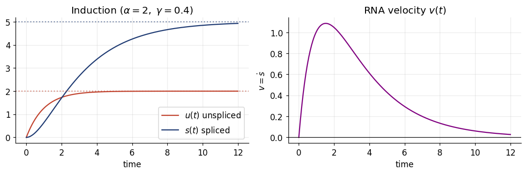
The two exponential time scales are the important part. Unspliced RNA responds on the scale $1/\beta$, while spliced RNA responds on the scale $1/\gamma$. When splicing is faster than degradation, the unspliced pool reacts first and the mature pool follows. RNA velocity reads precisely this lag.

The phase portrait

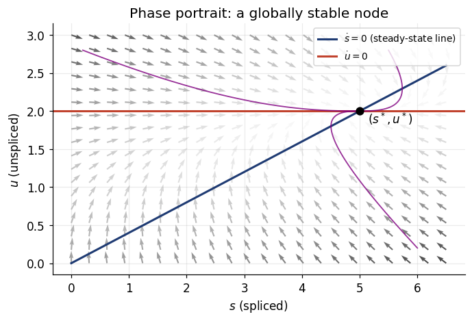
The geometry is easiest to see in the $(s,u)$ plane, with spliced abundance on the horizontal axis and unspliced abundance on the vertical axis. The two nullclines are

and

Their intersection is the fixed point

The Jacobian is constant:

Because it is triangular, its eigenvalues are visible on the diagonal:

Both are real and negative. The fixed point is therefore a stable node; because the original system is affine linear, this local calculation is also global. For a fixed $\alpha$, every initial condition is drawn to the same equilibrium. That’s a very good thing from the perspective of a cell – while mRNA is continuously being generated and degraded, this stability ensures that for fixed $\alpha, \gamma, \beta$ one attains a stable homeostasis for the expression of a desired gene. If this behaved differently, i.e. with unstable equilibria, I’d frankly be quite concerned…

Show the nullcline and stability calculations line by line.

Switching transcription creates the loop

A single fixed point does not yet look much like biological development. The characteristic RNA-velocity loop appears when transcription switches.

In the simplest dynamical model, a gene has two phases that share $\beta$ and $\gamma$:

1. Induction: $\alpha=\alpha^{\mathrm{on}}>0$, beginning near $(u,s)=(0,0)$.
2. Repression: $\alpha=0$, beginning from the state reached at a switching time $t_s $.

During induction, the unspliced pool runs ahead of the mature pool. The state lies above the steady-state line and $\dot s>0$. Once transcription turns off, unspliced RNA is depleted first while mature RNA lingers. The state falls below the line and $\dot s<0$. Together the two branches trace an almond-shaped loop.

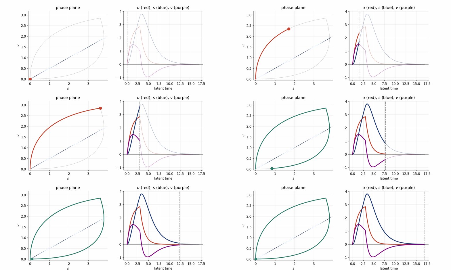
This is why a cross-section of many cells can stand in for time – the model assumes that different cells occupy different points along a common kinetic curve in the phase plane. Inference then asks where each cell sits on that curve and which kinetic parameters generated it.

Velocity is a signed residual

The key geometric fact is almost embarrassingly simple. Starting from

we can factor out $\beta$:

After setting $\beta=1$,

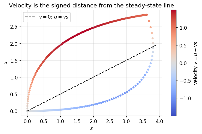
The steady-state line is $u=\gamma s$. At a fixed value of $s$, its vertical coordinate is $\gamma s$, so $u-\gamma s$ is exactly the signed vertical gap between the observed cell and the line:

The perpendicular distance differs by the positive factor $1/\sqrt{1+\gamma^2}$, so it carries the same sign. In this phase portrait, “RNA velocity” is a residual from a line.

Show the signed-distance calculation.

Estimating velocity from cells

The equations tell us how to compute velocity if the rates are known. The statistical problem is to infer those rates from an unordered cloud of measured cells.

The steady-state estimator

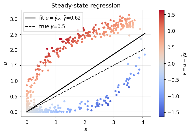
The original approach fixes $\beta=1$ and estimates the slope $\gamma$ from cells thought to lie near steady state. In a schematic least-squares version, choose the high-expression cells and solve

Differentiating gives the closed-form slope through the origin,

Show the least-squares derivative and normal equation.

This is fast and intuitive, but it assumes the extreme cells actually reached steady state. While this was the core of the initial approaches to RNA velocity, it is a less-than-ideal assumption for two reasons:

1. The cells may not be in steady state. Developmental processes are often transient: a gene can switch off before its induction trajectory reaches the asymptote. In that case, the upper cells lie on the curved part of the loop and the fitted slope is biased.

2. It fits only these extremal cells, which discards much of the data.

Fitting the whole dynamical curve

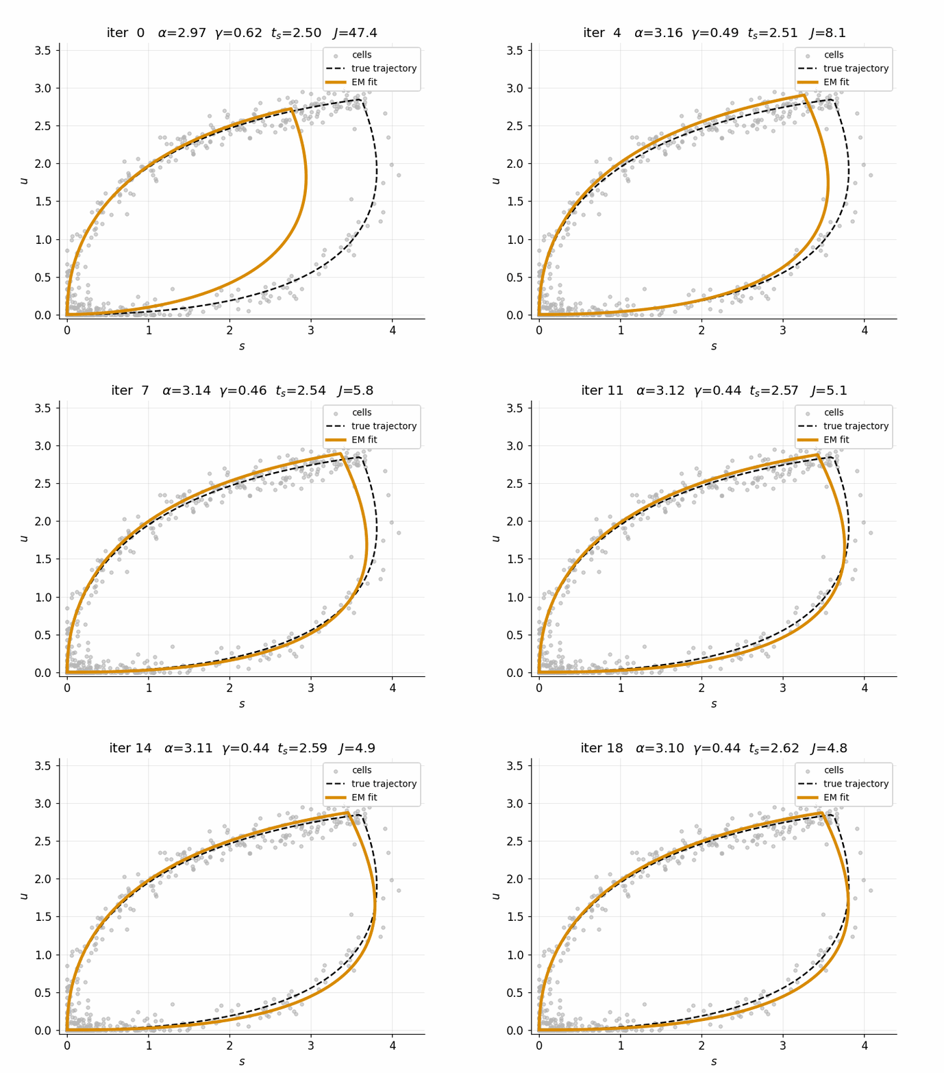
The scVelo dynamical model addresses this transient regime by fitting the full induction/repression trajectory. For one gene, let

denote the shared kinetic parameters. Every observed cell $i$ receives hidden coordinates

where $t_i$ is its latent transcriptional time and $k_i$ selects the induction or repression branch. The closed-form solution predicts a point

on the phase curve.

A useful pedagogical observation model is isotropic Gaussian noise around that curve:

Maximum likelihood is then equivalent to minimizing the total squared distance

The simplified hard-assignment EM procedure in the notebook alternates between two geometric operations:

• E-step: hold $\theta$ fixed and project each cell to its nearest point on the current curve.
• M-step: hold the cell assignments fixed and deform the curve by updating $\theta$.

Each operation can only lower the objective:

The objective therefore converges, although the non-convex problem may have multiple stationary points. A soft probabilistic version keeps a posterior distribution over latent times and phases instead of assigning each cell to a single point.

Show how the Gaussian likelihood gives the objective and why hard EM decreases it.

From genes to a cell-state vector field

For $p$ genes, a cell’s spliced transcriptome is a point

and its gene-wise velocities form the vector

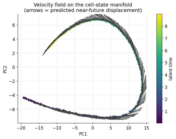
Cells tend to concentrate near a much lower-dimensional manifold $\mathcal M\subset\mathbb R^p$. If the kinetic model is a useful description, $v_i$ is approximately tangent to $\mathcal M$ at $x_i$. The collection of inferred velocities is therefore a discrete sampling of a vector field over cell state.

To visualize the field, the attached notebook predicts a short Euler step

and applies the same linear PCA map $Q$ to both states. Linearity gives

so each displayed arrow is the projected near-future displacement.

One can turn this field into a stochastic process on the cell graph. For neighboring cells $i$ and $j$, reward displacements that align with $v_i$:

Row normalization makes $P$ a Markov transition matrix. Methods such as CellRank analyze this chain to identify terminal states and compute fate probabilities as absorption probabilities.

What the snapshot cannot identify

There is a fundamental ambiguity in the inverse problem. Choose any $c>0$ and transform

The combinations $\beta t$, $\gamma t$, $\alpha/\beta$, and $\alpha/\gamma$ do not change, so neither does the trajectory in the $(u,s)$ plane. Equivalently, if $t’=t/c$, then

and similarly for $s$. The same curve can be traversed at any absolute speed, provided all rates are rescaled together.

Show the time-rescaling argument directly in the closed-form trajectory.

Snapshot splicing data can therefore determine the shape and orientation of a trajectory, along with dimensionless ratios such as $\gamma/\beta$, but it cannot supply an absolute clock. The sign and relative magnitude of velocity are meaningful; i.e. “molecules per hour” is not identifiable from these measurements alone.

Absolute kinetics require another source of time information. Metabolic labeling time-stamps newly synthesized RNA, which is why methods such as Dynamo can estimate absolute velocity and reconstruct an analytic vector field.

The picture to keep

RNA velocity works by turning a biochemical lag into geometry:

1. Transcription, splicing, and degradation define a two-state kinetic system for every gene.
2. Switching transcription on and off creates a loop around the steady-state line.
3. A cell’s signed displacement from that line estimates $\dot s$.
4. Gene-wise derivatives assemble into a vector field over the cell-state manifold.
5. That field induces a Markov chain and, downstream, probabilities over cellular fates.

The surprising step is the first one: a destructive snapshot still contains temporal information because RNA processing does not happen instantaneously. Everything after that is the mathematical work of making this internal clock visible.

Further reading

• Gioele La Manno et al., RNA velocity of single cells (2018).
• Volker Bergen et al., Generalizing RNA velocity to transient cell states through dynamical modeling (2020).
• Marius Lange et al., CellRank for directed single-cell fate mapping (2022).
• Xiaojie Qiu et al., Mapping transcriptomic vector fields of single cells (2022).

Appendix: informal calculations

This appendix keeps the scratch-work version of the derivations: no steps hidden, and no need to interrupt the main narrative if the result already feels intuitive.

• A. Solving the kinetic equations
• B. Nullclines, equilibrium, and stability
• C. Velocity as a signed distance
• D. The steady-state regression
• E. The dynamical model and hard EM
• F. Identifiability under a change of clock

A. Solving the kinetic equations

Start from

with $u(0)=u_0$ and $s(0)=s_0$.

The unspliced pool

Move the decay term to the left:

Multiplication by $e^{\beta t}$ makes the left side a product derivative:

Integrating from $0$ to $t$,

Now divide by $e^{\beta t}$:

Writing $u_\infty=\alpha/\beta$, this is

The spliced pool

Now substitute the solution for $u(t)$ into

Multiplying by the second integrating factor $e^{\gamma t}$ gives

For $\gamma\neq\beta$, integration from $0$ to $t$ yields

Because $\beta u_\infty=\alpha=\gamma s_\infty$, we have $\beta u_\infty/\gamma=s_\infty$. Multiplying through by $e^{-\gamma t}$ therefore gives

Thus

If $\gamma=\beta$, the second integrand above becomes constant:

Its integral is $t$, so the resonant solution is

This is also the limit of the non-resonant expression as $\gamma\to\beta$.

Switching from induction to repression

Set $\beta=1$. During induction, $\alpha=\alpha^{\mathrm{on}}$ and $(u_0,s_0)=(0,0)$. Substitution into the closed-form solutions gives

and

At the switching time $t_s$, define

During repression $\alpha=0$, so both steady-state values vanish. With elapsed repression time $\tau=t-t_s$, the same general solution gives

and

Those two pieces are the upper induction branch and lower repression branch of the loop. Return to the kinetic discussion.

B. Nullclines, equilibrium, and stability

The $u$-nullcline is found by setting $\dot u=0$:

Along this horizontal line,

so the horizontal component of the flow points toward $s=\alpha/\gamma$.

The $s$-nullcline follows from

or, in the axes used in the figures,

The two nullclines meet at

For the stability calculation, write the vector field as

Differentiating each component gives

The characteristic polynomial is

Therefore

Since $\beta,\gamma>0$, both modes decay. If we shift to deviations from equilibrium,

then the affine term disappears and the exact equation is $\dot y=Jy$, not merely an approximation near the fixed point. Hence $y(t)=e^{Jt}y(0)\to0$, and the equilibrium is globally asymptotically stable. The two decay scales are $1/\beta$ and $1/\gamma$. Return to the phase portrait.

C. Velocity as a signed distance

Begin with the definition

Factor out $\beta$:

The $\dot s=0$ nullcline is

For an observed point $(s,u)$, the point on this line with the same horizontal coordinate is

Their signed vertical difference is

Thus the vertical residual equals velocity after choosing the time unit $\beta=1$; for general $\beta$, it differs only by the positive scale factor $\beta$.

For completeness, the line can be written as

The signed perpendicular distance from $(s,u)$ to this line is

Every factor in the denominator is positive, so vertical residual, perpendicular distance, and velocity always have the same sign. Return to the velocity geometry.

D. The steady-state regression

After setting $\beta=1$, suppose a selected group of cells is close enough to steady state that $u_i\approx\gamma s_i$. Fit a line through the origin by minimizing

Differentiate one term at a time:

At the optimum, $J’(\widehat\gamma)=0$, so

Provided at least one selected cell has $s_i\neq0$,

The second derivative is

so this stationary point is the unique minimum. Substituting the fitted slope back into the kinetic equation produces

The algebra is exact; the vulnerable step is the biological assumption that the selected cells really lie near the steady-state line. Return to the steady-state estimator.

E. The dynamical model and hard EM

Let $y_i=(u_i,s_i)$ be an observed cell and let $z_i=(t_i,k_i)$ contain its latent time and branch. Given kinetic parameters $\theta$, the model curve predicts $m(z_i;\theta)$. Under isotropic Gaussian observation noise,

Assuming the cells are conditionally independent,

Taking logarithms turns the product into a sum:

The first term does not depend on $Z$ or $\theta$. Maximizing likelihood is therefore equivalent to minimizing

For a hard E-step, fix $\theta^{(r)}$. Each latent assignment can be optimized separately:

Geometrically, this projects every cell onto its nearest point on the current trajectory. Since $Z^{(r+1)}$ minimizes over the assignments while $\theta^{(r)}$ stays fixed,

For the M-step, fix the new assignments and update the kinetic parameters:

Therefore

Combining the two inequalities gives

The sequence of objective values is monotone and bounded below, so those values converge. This does not imply a unique fitted parameter vector: the problem is non-convex, and the time-rescaling symmetry below creates an additional ambiguity. A soft EM treatment replaces the nearest-point assignment by a posterior distribution over $z_i$. Return to the dynamical estimator.

F. Identifiability under a change of clock

Take any $c>0$ and define rescaled rates

Evaluate the primed system at the rescaled time $t’=t/c$. Its steady-state values are unchanged:

and

The exponents are also unchanged:

Substitution into the unspliced solution gives

For the spliced solution, the remaining coefficient is invariant as well:

Consequently,

The same point in the phase plane is therefore generated by rates $(\alpha,\beta,\gamma)$ at time $t$ and by rates $(c\alpha,c\beta,c\gamma)$ at time $t/c$.

The chain rule expresses the same fact directly at the ODE level. Since $t’=t/c$, we have $dt/dt’=c$, and hence

with the identical calculation for $s$. Snapshot observations see the curve but not the speed at which it is traversed. They can identify ratios such as $\gamma/\beta$, not the common rate scale. Return to the identifiability discussion.